





How to Read a DC Blower Fan Curve and Find the Real Operating Point
A DC blower fan curve shows how much airflow a blower can deliver at different static-pressure loads. It is not a promise that the blower will produce its maximum airflow after installation. The real airflow is found where the blower’s pressure–airflow curve intersects the resistance curve of the enclosure, duct, filter, heat sink, or other connected system. That intersection is the operating point.
What a DC Blower Fan Curve Actually Shows
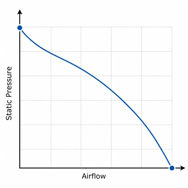
A typical P–Q curve plots airflow, or Q, on the horizontal axis and static pressure, or P, on the vertical axis. Airflow may be stated in CFM, m³/h, or m³/min. Static pressure may be stated in Pa, mmH₂O, or in. w.g. Always confirm the units before comparing two products.
The curve belongs to a particular blower model under stated test conditions: normally a specified voltage, speed, air density, and inlet/outlet arrangement. A curve measured at one voltage or speed cannot be applied unchanged to another operating condition.
The left end represents shutoff: the outlet is blocked, airflow is approximately zero, and the blower develops its maximum static pressure. The right end represents free delivery: system resistance is approximately zero, static pressure is zero, and airflow is at its maximum. Neither endpoint is normally the desired design condition.
Why Maximum Airflow Is Not Installed Airflow
Maximum airflow is measured near zero external resistance. Once the blower is installed, every grille, filter, bend, heat exchanger, narrow passage, cable bundle, and outlet opening produces a pressure loss. The blower must generate enough pressure to overcome the combined loss before air can move through the assembly.
This is why two enclosures using the same blower can have different airflow. The blower curve has not changed, but the system curves are different. A compact enclosure with a dense filter and several turns generally has a steeper resistance curve than an open enclosure with a short, straight flow path.
The System Curve and the Real Operating Point
A system curve describes the pressure loss produced by the complete air path at different flow rates. For many turbulent-flow systems, pressure loss varies approximately with the square of airflow. If one measured or calculated duty point is known, a simplified system curve can be estimated with ΔP₂ = ΔP₁ × (Q₂/Q₁)², provided the geometry and flow regime remain comparable.
Plot the system curve on the same axes and in the same units as the blower curve. Where the two curves intersect, blower pressure equals system pressure loss. The coordinates of that point give the airflow and static pressure the installed system will settle at.
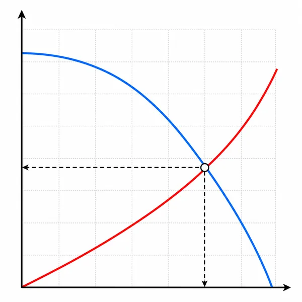
The operating point is a balance, not a setting entered into the blower. If resistance increases, the system curve rises and the intersection moves toward lower airflow and higher pressure. If resistance decreases, the point moves toward higher airflow and lower pressure.
Visual Guide: Understanding Fan P-Q Curve and Operating Point
How to Read a Blower Curve Step by Step
- Confirm the exact model and conditions. Check rated voltage, speed, air density, temperature, and test configuration.
- Identify both axes and units. Do not compare Pa with mmH₂O or CFM with m³/h without conversion.
- Mark the required airflow. Determine the flow needed for heat removal, ventilation, process delivery, or another engineering target.
- Estimate pressure loss at that flow. Add the losses of filters, heat sinks, ducts, grilles, bends, and other components using supplier data or measurements.
- Plot the duty point. Mark required airflow and estimated system pressure on the blower graph.
- Check whether the point lies below the blower curve. A required point above the curve cannot be achieved at that speed and condition.
- Draw or calculate the system curve. The actual intersection, not the isolated duty-point marker, predicts the operating airflow.
- Keep engineering margin. Allow for filter loading, tolerances, dust, voltage variation, temperature, manufacturing variation, and aging without selecting an unnecessarily oversized blower.
A Simple Operating-Point Example
Assume an enclosure loses 80 Pa at 20 CFM. If its loss follows the square-law approximation, the estimated loss at 30 CFM is 80 × (30/20)², or 180 Pa. Plotting several calculated points creates the system curve. If the blower curve intersects it at 25 CFM and 125 Pa, then 25 CFM—not the blower’s free-air value—is the estimated installed airflow.
This method is more useful than asking whether a blower is “rated for 30 CFM.” A free-air rating does not show whether the product can maintain 30 CFM against the enclosure’s required pressure.
How Filters and Duct Changes Move the Point
Adding a filter raises resistance. A dirty filter usually raises it further. Smaller openings, longer ducts, sharp elbows, obstructed inlets, and abrupt outlet transitions have a similar effect. On the combined graph, the new system curve becomes steeper and intersects the same blower curve at lower airflow.
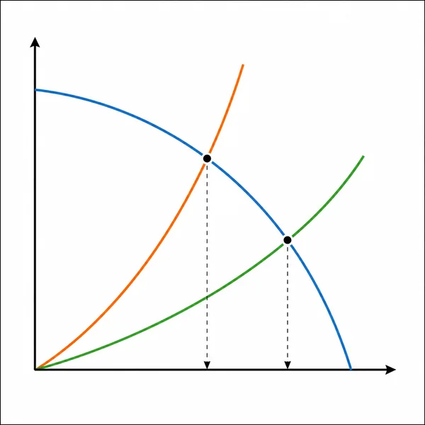
The opposite is also true. Increasing the effective vent area, improving inlet clearance, using smoother transitions, or reducing unnecessary bends lowers the system curve and can recover airflow without changing the blower.
Common Mistakes When Using a P–Q Curve
Using only the maximum CFM value
Maximum airflow describes the zero-pressure endpoint. It is rarely the installed condition and should not be used alone for thermal design.
Using only maximum static pressure
Maximum pressure occurs at approximately zero airflow. A blower cannot deliver both maximum airflow and maximum static pressure simultaneously.
Adding component pressure losses at the wrong flow
A filter’s loss at 20 CFM cannot be added directly to a heat sink’s loss specified at 40 CFM. Normalize or obtain all losses at the same target airflow.
Ignoring inlet and outlet system effects
A blocked inlet, outlet placed against a wall, sudden expansion, or poorly aligned duct can cause losses that are absent from component datasheets. AMCA refers to additional installation-related loss as system effect.
Assuming every curve uses standard air
Air density changes with temperature, altitude, and composition. Pressure capability and power requirements may need correction when operating conditions differ materially from the published test basis.
Speed, Voltage, and the Fan Laws
For geometrically similar operation within an appropriate range, airflow varies approximately with rotational speed, pressure varies with the square of speed, and power varies with the cube of speed. A 10% speed increase therefore does not simply add 10% pressure or power. Actual electronically commutated DC blowers also have motor, controller, current, and thermal limits, so manufacturer curves at the intended command or voltage are preferred over extrapolation.
Do not scale a 12 V curve to 24 V unless the product is designed for that voltage and the manufacturer permits the method. The YCCFAN DC blower fan range includes different sizes and electrical configurations; selection should use the curve for the exact model and operating condition.
How to Validate the Selected Operating Point
Curve analysis is a design prediction. Validate the assembled system by measuring airflow or a correlated parameter, pressure differential, current, temperature, and acoustic behavior. Test with covers installed and the intended filter, grille, duct, and heat source in place. Repeat the test at expected voltage and temperature extremes and with a representative loaded filter.
If measured airflow is lower than predicted, check for leakage, recirculation, inlet starvation, incorrect polarity, unexpected restrictions, measurement location, and differences between the test setup and the published curve. Do not immediately replace the blower before checking the air path.
Authoritative References
AMCA explains that the system curve and fan curve intersect at the operating point in its fan curve engineering guide. The ebm‑papst fan performance FAQ likewise defines the operating point as the intersection of fan performance and system resistance. These principles apply to compact DC centrifugal blowers as well as larger air-moving systems.
Frequently Asked Questions
What does P–Q mean on a blower curve?
P is pressure and Q is volumetric airflow. The curve shows the pressure the blower can develop at each flow rate under the stated test conditions.
Can I use the free-air CFM value for enclosure cooling?
No. Use the intersection of the blower curve and the enclosure system curve. Filters, heat sinks, grilles, and internal geometry reduce installed airflow.
How much margin should I add?
There is no universal percentage. Margin should reflect filter loading, component tolerances, operating temperature, voltage range, aging, and the consequence of insufficient cooling. Verify the design with testing rather than relying only on oversizing.
Why can a higher-pressure blower still deliver less airflow?
Pressure and airflow must be compared at the same operating point. A blower with a higher shutoff pressure may have a different curve shape and may not provide more airflow at the system’s actual resistance.
Conclusion
Read a DC blower fan curve as a relationship, not as two independent maximum ratings. Build or estimate the system curve, place it on the same P–Q chart, and use the intersection to predict real airflow. Then validate the complete installed system. For model-specific curve data, connector options, and operating conditions, contact the YCCFAN engineering team.